Exploratory Data Analysis (EDA)

Exploratory Data Analysis (EDA) is an approach to analyzing data sets to summarize the data, using statistical analysis and data visualization methods.

It is a crucial step in any data analysis process, enabling data analysts to uncover patterns, spot anomalies and gain insights to take actions

Here is video pesentation to Euromart:

About the company

• Euromart is a retail store having its chain of operating stores across Europe in 15 counties
• They offer variety of product categories to the customers
• Euromart wants to leverage its transactions data to improve its business
• Euromart have reached Certisured for their requirements

Problem Statement & Objective

Problem Statement: 

Identify key factors influencing sales and profitability in different regions, product categories, and transaction types to optimize operations and pricing strategies.

Objectives

Identifying Top Performers: Pinpoint regions, product categories, and transaction types driving highest sales & profitability to replicate successful strategies.

Understanding Challenges: Address operational inefficiencies and customer engagement issues in underperforming areas.

Optimizing Discounts & Shipping Modes: Analyze the impact of discounts and shipping modes to refine pricing strategies and logistics for max profitability.

Leveraging Customer Feedback: Use customer feedback to enhance product offerings and improve overall business performance.

Improving Product Mix: Identify top-selling products and customer preferences to optimize our product mix.

Attached the PDF report for refrence(to download):

Source file of excel for download: https://docs.google.com/spreadsheets/d/1Vzn4IwA8pQecqq6zxmc46Dqcu0M6n0dJ/edit?usp=sharing&ouid=101747674571343340244&rtpof=true&sd=true

Github link: https://github.com/VenuKumarM1/Euromart

Python file for download: https://github.com/VenuKumarM1/Euromart/blob/main/Euro_Mart_Venu%20Kumar_Final.ipynb

Download the report from the above attachment 🙂

EDA Pipeline

1. Data Acquisition and Objective
   • Obtain Euromart data (CSV, Excel)
   • Get problem statement from Euromart
   • Choose tools/environment & programming language
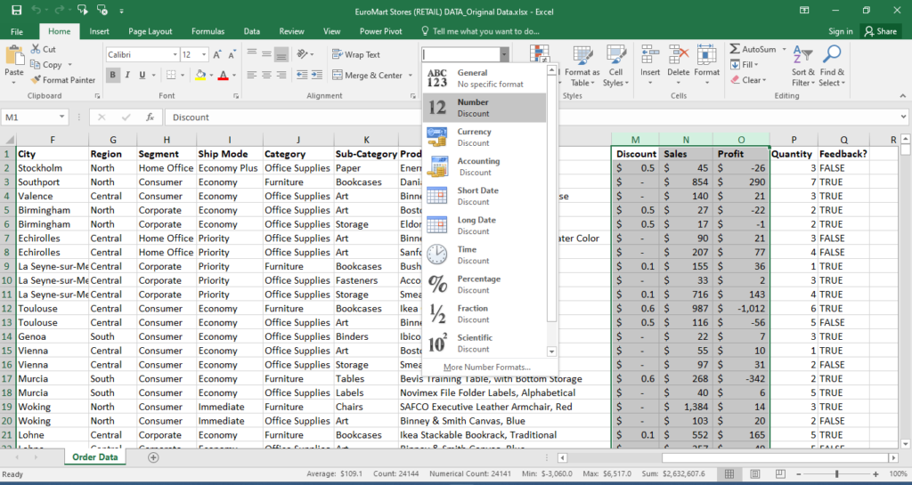
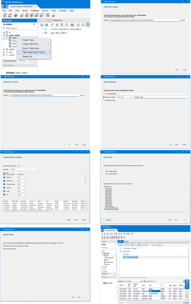
2. Data Loading/Reading   
   • Load data in MySQL (Remove duplicates)
   • Load data in Jupyter Notebook/VS Code (To perform further analysis)
3. Familiarize with Data & Identify Target Variable
   • Explore data (column names, data types)
   • Identify target variable based on objective
4. Data Preparation & Transformation
   • Data Cleaning
   • Handle missing values (imputation, deletion)Removal of unwanted data (if present)
   • Format data types (numerical & categorical)
5.  Feature Engineering (Create new features)
6. Data Analysis & Visualization
   • Univariate Analysis
     • Numerical variables (mean, median, stddev)Categorical variables (distribution)
   • Bivariate & Multivariate Analysis (Identify patterns)
     • Visualization (Charts: pie, boxplot, histogram, heatmap)
7. Summary and Suggestions

Tools and platforms used in project

Why Python and MYSQL?

Python is a high level and open source programming language for mathematical computations and basic visualizations. SQL is the most common language for querying relational databases. Also, Python and SQL are most sought after programming languages in the India today

Platforms used

• Jupyter notebook – it is a web-based application for running code and queries in Python
• Visual Studio Code (VS Code) – it is a free, opensource code editor which supports multiple programming languages
• MySQL – MySQL workbench by Oracle is widely used open-source RDBMS, it is cross-platform support

Versions of platform

• Jupyter notebook – 7.1.3
• Visual Studio Code – 1.89.1
• MySQL Workbench – 8.0.36
• Python version – 3.12.2

Note: Code format is IPYNB file.It is a text-based file used by Jupyter Notebook (VS Code also supports IPYNB with Jupyter extension)

Chapter 1: Data Loading/reading

Load Data in MySQL

We need to import necessary libraries for performing loading, connecting with SQL and doing analysis

Import Necessary Library

• mysql.connector: Library offers connectivity to MySQL server to query from database
• numpy (np): Provides efficient numerical computation tools
• pandas (pd): Offers data manipulation and analysis structures (DataFrames, Series)
• seaborn (sns): Creates informative statistical data visualizations based on Matplotli
• matplotlib.pyplot (plt): Enables various plot creations for data visualization
• %matplotlib inline (Jupyter Notebook specific): Displays plots within the notebook
• warnings (with warnings.filterwarnings(“ignore”)): Suppresses warnings

Establish a connection to the Euro Mart database using MySQL Connector

• Initialize a connection to a MySQL database named euro_mart on the local machine (localhost).
• Uses credentials with username and password

Load Data (Jupyter Notebook or VS Code) from MySQL

The data is loaded to Jupyter Notebook from MySQL, this actively removes all the null values in rows by default, which is make data one step closer for it to be cleaned

Retrieve data from a MySQL database table and load it into a pandas DataFrame for further analysis in Jupyter Notebook

• query1 = “Use euro_mart; establishes connection with correct database
• query = “select * from euromart_table; selects all columns (*) from the table named euromart_table
• df = pd.read_sql(query, Connection); execute the defined query (query) on the established connection (Connection). The result is stored in a pandas DataFrame named df

Chapter 2: Familiarize with Data & Identifying the Target Variable

Explore the provided data (column names, data types)

• We need to understand the data before cleaning the data and also cross verify if all the required data are provided by Euromart

Overview of data

• df.head(); Let’s see the data by displaying the first 5 rows
• df.tail(); Let’s see the last 5 rows
• df.shape is used to get the dimensions (number of rows and columns) of data
• df.size is used to get the total number of elements in a pandas
• df.info() – used to display concise information about

Interpretation

• Structured Data: Data provided is in table format
• Dimensions (17 Columns x 8047 Rows, and has 1,36,799 elements in it) of the DataFrame or data
• Column Data Types: Observed mix of data type of each column (e.g., object, float, int, etc.)
• Also note that all categorical/qualitative variables are Nominal in nature (it has no specific orders)
• Non-Null Counts (no Null values observed) in each column.
• Memory Usage: An estimate of the memory usage is 1.0+ MB (Further, we will optimize the memory usage by modifying the data types)

Chapter 3: Data Preparation & Transformation

Data Cleaning

We need to perform steps mentioned below to clean data:

• Steps involved in handling missing values (imputation, deletion)
  • We accept missing values if data is small in dimension
  • We delete missing values if:
    • When more than 80% of data is missing/null values
    • When the percentage of missing values are very small, deleting will have minimal effect on analysis
• Replacing the missing values by imputation
  • Imputation: We replace the missing values by Mean, Median or Mode of the variable or perform fill null values(fillna method) with the desired value
• Data Reduction: Remove unwanted data (if present) which are not required for analysis
  • Delete unwanted columns
  • Delete duplicate rows
• Format data types (numerical & categorical variables)
• Outlier detection and handling (we ignore this step because outliers are valid in our case)
  • When data has extreme values that could effect our analysis, we either replace them with Mean or Median or Mode values or we accept the outliers
  • We identify the outliers by plotting the Box plot

Handle missing values (imputation or deletion)

• df.isnull().sum() – Gives sum of all null values in each column
• df.notnull().sum() – Gives sum of all not null unique values in each column
• Interpretation:
  • Data has no null values, so no need to perform process to handle missing values

Data Reduction: Remove unwanted columns or rows

There are no unwanted columns to delete, so we can check for duplicated rows and delete the duplicates

• df.duplicated().sum(); This shows number of duplicated rows
• df = df.drop_duplicates(); This removes duplicated rows
• Interpretation:
  • It is noted that there are 2 rows which are repeated. We have removed duplicated rows

Format data types (numerical & categorical)

We need to format columns, that will ease data analysis, below steps are performed to the required format for analysis

• Rename of columns – To keep columns descriptive as well as simple
• Change data types – We change data type to keep consistency and also for memory optimization

Rename of columns

• df.rename(columns={‘Feedback?’: ‘Feedback’}, inplace=True) – This renames the column name, Inplace=True; this permanently alters the name
• df.columns; This display columns for cross verifying that renaming step is performed
• Interpretation:
  • Feedback column is renamed by removing special character in column

Change data types of columns and Memory optimization

• df.info(); We can see the column data type
• cols_to_convert = df.columns[2:12]; Select 3rd column to 12 column
• df[‘Order Date’] = pd.to_datetime(df[‘Order Date’]); Convert the “Order Date” column to datetime data type
• Interpretation:
  • We are converting all columns with object data type to category and converted order date column to date-time format
  • Now memory usage is reduced from 1.0+ MB to 700+ KB. With this we achieved memory optimization for space complexity

Feature Engineering (Create new features/variables)

• We derive new variables or features by combining multiple columns or derive new features by performing calculation
• Here we need to create new columns for easier analysis
• Create new columns by extracting date, month, year and generate new columns like Quarter and Weeks
• Create new columns by calculating Total sales, Total profit, Profit margin and discount percentage

Create new features

• df[‘Year’] = df[‘Order Date’].dt.year; Extract and create a new column named Year form Order date column
• df[‘Month’] = df[‘Order Date’].dt.month; Extract and create a new column named Date form Order date column
• df[‘Day’] = df[‘Order Date’].dt.day; Extract and create a new column named Year Day Order date column
• quarter_dict = {1 : ‘Q1’, 2 : ‘Q1’, 3 : ‘Q1’,4 : ‘Q2’……}; this defines a dictionary which maps month to corresponding Quarters
• df[‘Quarter’] = df[‘Month’].map(quarter_dict); this uses the map method to apply the quarter_dict dictionary to the “Quarter” column
• week_dict = {1: ‘W1’, 2: ‘W1’, 3: ‘W1’……}; this defines a dictionary which maps days to corresponding Week
• df[‘Week’] = None; Initialize ‘Week’ column with None values
• df[‘Week’] = df[‘Day’].map(week_dict); this uses the map method to apply the week_dict dictionary to the “Week” column
• df.info; gives list of all columns and its details for cross verifying on feature engineering
• df[‘Order Size’] = df.groupby(‘Order ID’)[‘Product Name’]; Create a new column based on number of times order ID is reapeated
• Interpretation:
  • We are set with feature engineering by creating multiple columns for easier analysis

Chapter 4: Data Analysis & Visualization

Overview of data before analysis

• After Data Wrangling, we can check the columns once before we proceed to perform analysis
• df.columns; Display all columns in the data frame
• Interpretation:
  • Description of variables

Variables/Columns	Description
Order ID	Unique identifier for each sales transaction
Order Date	Date and time of the purchase
Customer Name	Name of the customer
Country, State, City, Region	Location of sales
Segment	Types of customers
Ship Mode	Shipping method chosen by the customer
Category & Sub-Category	Purchased product category and more specific sub category
Product Name	Name of the specific product purchased
Discount and Discount Percentage	Discount applied to the purchase (if any)
Sales	Total sales amount for the transaction
Profit	Profit earned on the transaction
Quantity	Quantity of each product purchased in the transaction
Feedback	Customer provided feedback on the purchase experience (binary)
Year, Month, Day, Week, Quarter	Extracted from Order Date
Total Sales	Sales for all items in a transaction (Product of sales and Quantity)
Total Profit	Profit for all items in a transaction (Product of Profit and Quantity)
Profit Margin	Profit margin per transaction (Total profit over total sales in percentage)
Order Size	Gives number of times the order is placed w.r.t order ID

Univariate analysis

We need to perform univariate analysis on relevent columns in Euromart data for more targetted approach

Summary statistics

• df.describe().T; We generate summary statistics for numerical columns in data df. and transpose the output
• Interpretation:
• Summary statistics provide valuable insights of data distribution to understand our data better
• Notable Observations
• Discount: There are products with discounts from nil up to 85%
• Order Quantity: Range from single unit to 14 units
• Sales:Minimum sales value starts 3 USD
• Profit: Average profit from all transactions are in positive space at 35 USD. With average margin of 10%, which is clearly a good sign for Euro Mart

Note: Numerical summary stats on categorical variable in Euro Mart data set are not yielding any valuable insights

Unique elements in column

• df.nunique(); Counts the number of unique elements in each column
• Interpretation:
  • We got cardinality (number of distinct categories) within each column
  • Euro Mart operates in 15 countries. Offering 17 kinds of products category across 3 kinds of customers

Univariate Analysis of Categorical Columns

Distribution of countries

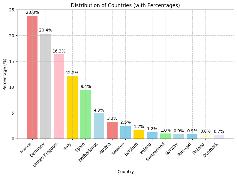
Distribution of countries

• France has the highest percentage at 23.8%, followed by Germany (20.4%), and the United Kingdom (16.3%)
• The other countries have progressively smaller percentages, with Denmark having the lowest at 0.7%
• France, Germany, and the United Kingdom are the most significant contributors to the Sales of EuroMart

Distribution of top 10 states

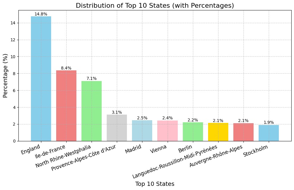
Distribution of top 10 states

• England has the highest percentage at approximately 14.8%, followed by Île-de-France at around 8.4% and North Rhine-Westphalia by 7.1%
• The other regions have percentages decreasing from roughly 3.1% to about 1.9%
• England and Île-de-France are the most significant state contributors

Distribution of different customer segment

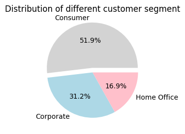
Distribution of different customer segment

• Consumer is the largest segment, likely accounting for around 51.9% of the total customers
• Corporate is the second largest segment contributing to 31.2%
• Home Office is the smallest segment, 16.9% of the customers

Distribution of different shipping modes

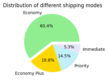
Distribution of different shipping modes

• Economy is the most used shipping mode, accounting for the largest portion, followed by Economy plus and Priority
• Immediate is the least used mode among the options presented

Distribution of different category of goods

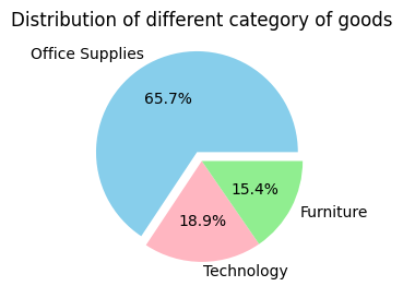
Distribution of different category of goods

• Office Supplies: This category constitutes the largest portion, accounting for 65.7% of the goods
• Furniture: Furniture makes up to 18.9% of the total
• Technology: The smallest segment is technology, representing 15.4%

Distribution of Top 5 Sub-Category of goods

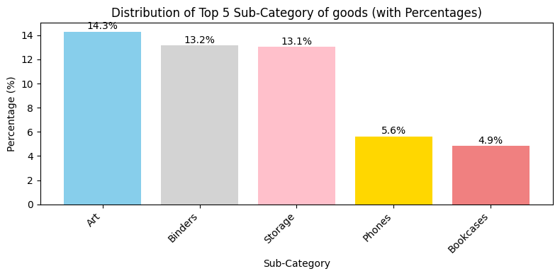
Distribution of Top 5 Sub-Category of goods (with Percentages)

• Art: This sub-category represents 14.3% of the goods
• Binders: Binders account for 13.2%
• Storage: The storage sub-category makes up 13.1%
• Phones: Phones have a smaller share of 5.6%
• Bookcases: Bookcases are the smallest segment, comprising for 4.9%

Distribution of feedback provided on purchase

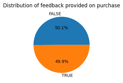
Distribution of feedback provided on purchase

• Almost half of the customers have given feedback on product purchase

Distribution of discount

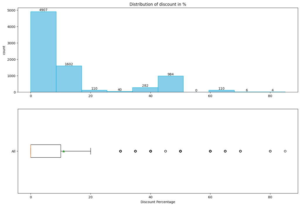
Distribution of discount

• There’s a significant spike in 0 to 20% discount range, indicating higher products presence in this discount range
• The box plot represents the interquartile range (IQR) with whiskers extending to show the range of discount percentages. Several outliers are visible beyond the whiskers
• Positively skewed distribution; here mean > median

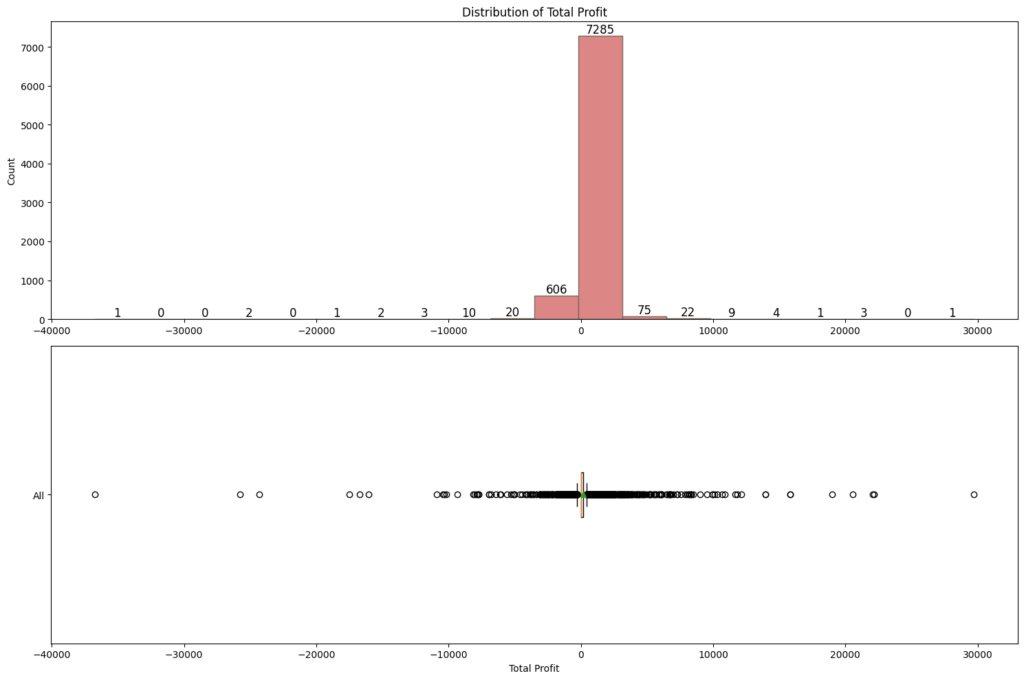
Distribution of total profit

Distribution of sales in month

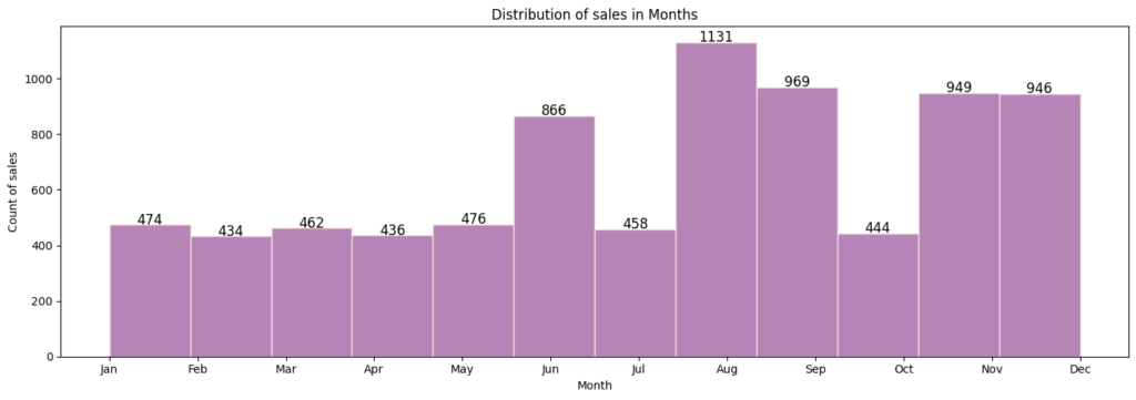
Distribution of sales in month

• Most of the sales happened in August, followed by September, November, December and June month
• First half of the year has low sales compared to next half of the year

Distribution of profit margin

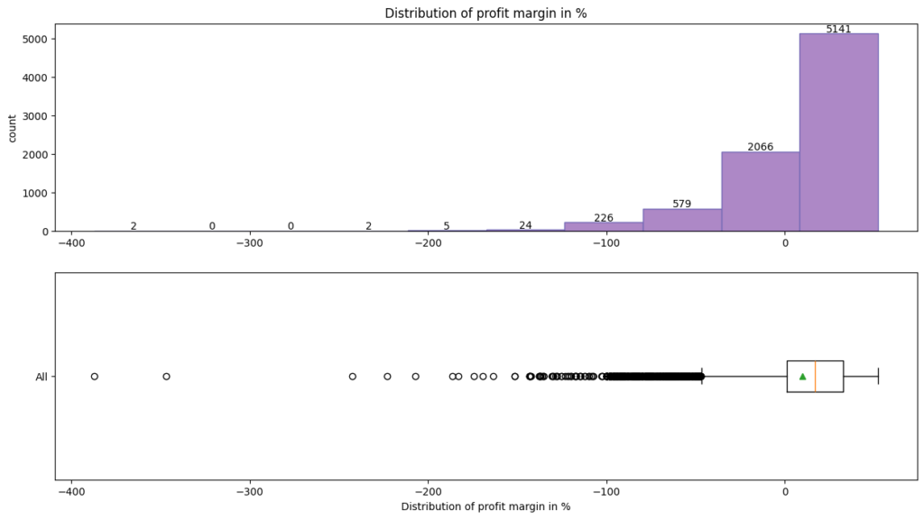
Distribution of profit margin

• Profit margin; Most bars cluster around the -100% to 0% range, suggesting a significant number of observations within this interval
• Fewer counts extend toward -300%, indicating less common occurrences
• Negatively skewed distribution; here, the mean < median

Distribution of sales in calendar days

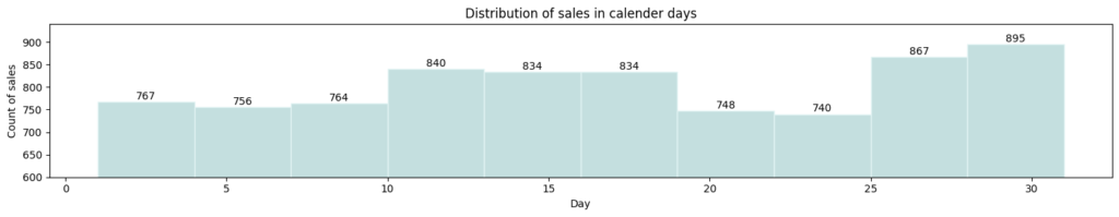
Distribution of sales in calendar days

• Most of the sales observed in month end from 25th to 31st calendar dates (Last 6 days) and followed by range of 10 to 20th calendar dates (Middle of month)

Distribution of quantity

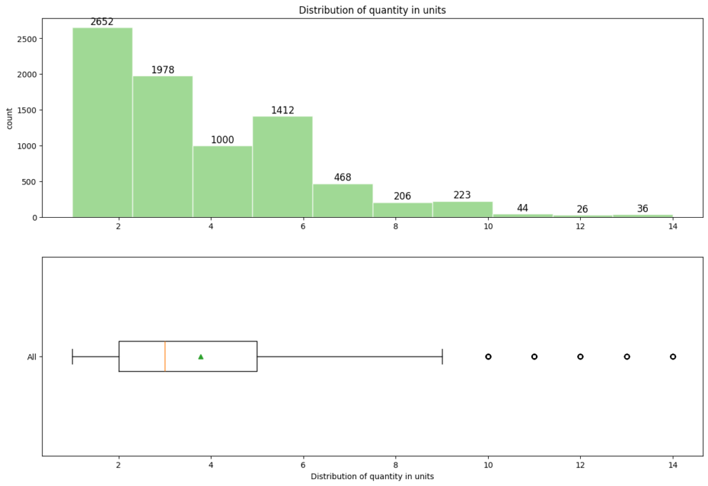
Distribution of quantity

• Sales quantity; most bars cluster around the 0 to 2 units range, indicating a higher occurrence of values within this interval
• Median is 3, Customers ordered most of the times 3 quantities in order
• Positively skewed distribution; here, the mean > median

Multivariate analysis

Identifying Top Performers

Correlation Heatmap of numerical variables

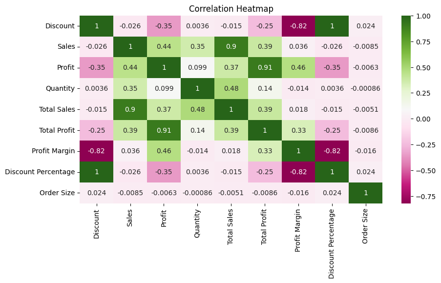
Correlation Heatmap of numerical variables

• Identifying potential relationships among target variables (Sales, Profit)
• We see that there is positive correlation among Sales, Profit and Quantity
• We are ignoring relation among Target variables (Sales, Profit) with Total sales, Profit margin, Discount percentage and Order size because those variables were derived from target variables

Target variables split by region

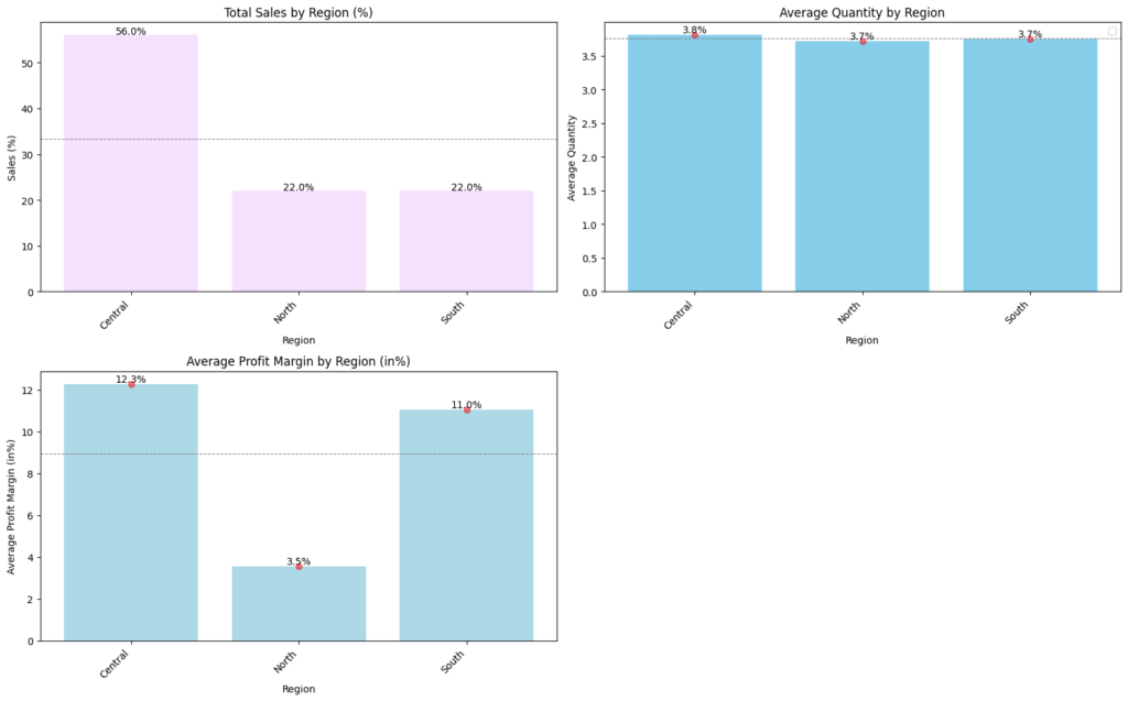
Target variables split by region

• Total Sales by Region: The Central region has the highest percentage of sales at 56.0%. North & South region both account for 22.2% of sales
• Average Quantity by Region: All regions show similar average quantities, hovering around 3.5 units
• Average Profit Margin by Region (%): Central and Soutth regions are contributing above the average profit margin compared to north region

Target variables split by country

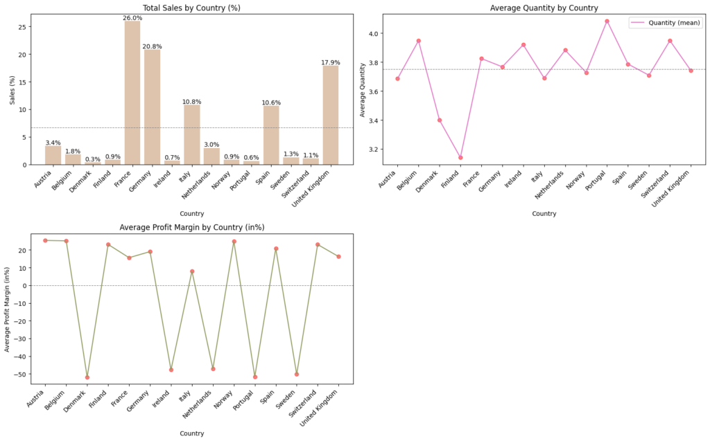
Target variables split by country

• Total Sales by Country: France, Germany, UK, Italy and Spain are having good sales contribution above the average sales among all the countries
• Average Quantity by Country: Order quantity ranges from 3 to 4 units among all country
• Average Profit Margin by Country (%): On average Euro Mart is incurring loss with negative profit margin in countries like Denmark, Ireland, Netherlands, Portugal and Sweden

Target variables split by states

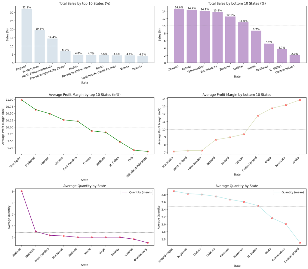
Target variables split by states

• Analysis by top 10 states
  • Total Sales by State:England, France, North Rihne-Westphalia are contributing to ~66% of top 10 states
  • Average Profit Margin by State(%):Top 10 states are contributing to positive profit margin above 9.25%. This is good sign for Euromart
  • Average Quantity by State:Average order quantity are in higher side ranging from 4.5 to 9 units
• Analysis by bottom 10 states
  • Total Sales by State:Zealand, Galway, Kymenlaakso, Extermadura, Zeeland & Setubal are contributing to ~80% of bottom 10 states
  • Average Profit Margin by State(%):Bottom 10 states are contributing to positive profit margin above 7%. This is good sign for Euromart
  • Average Quantity by State:Average order quantity are in lower side ranging from 1.5 to 3 units

Target variables split by cities

Target variables split by cities

• Analysis by top 10 Cities
  • Total Sales by Cities:London, Berlin, Vienna, Madrid, Paris are contributing to ~68% of top 10 Cities
  • Average Profit Margin by Cities(%):Top 10 Cities are contributing to positive profit margin range of 9.8% to 10.3%. This is good sign for Euromart
  • Average Quantity by Cities:Average order quantity are in higher side ranging from 8 to 12 units
• Analysis by bottom 10 Cities
  • Total Sales by Cities:Cestas, Ragusa, Battipaglia, Millau, Leiden, Friedenberg are contributing to ~80% of bottom 10 Cities
  • Average Profit Margin by Cities(%):Bottom 10 Cities are contributing to positive profit margin above 8.5%. This is good sign for Euromart
  • Average Quantity by Cities:Average order quantity are in lower side of only 1 unit. This is a concern for Euromart

Target variables split by consumer segments

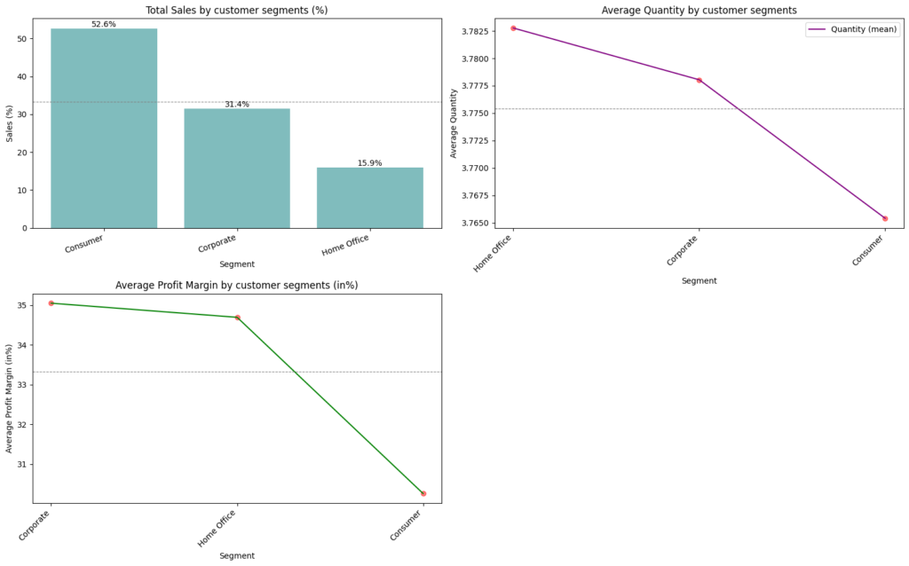
Target variables split by consumer segments

• Sales by Customer Segments (%): Consumers sales have contributed over 52%, followed by corporate and home office
• Average Profit Margin by Customer Segments(%): Profit margin stands in positive range from 30 to 35%
• Average Quantity by Customer Segments: Average quantity is nearly 4 units

Target variables split by category

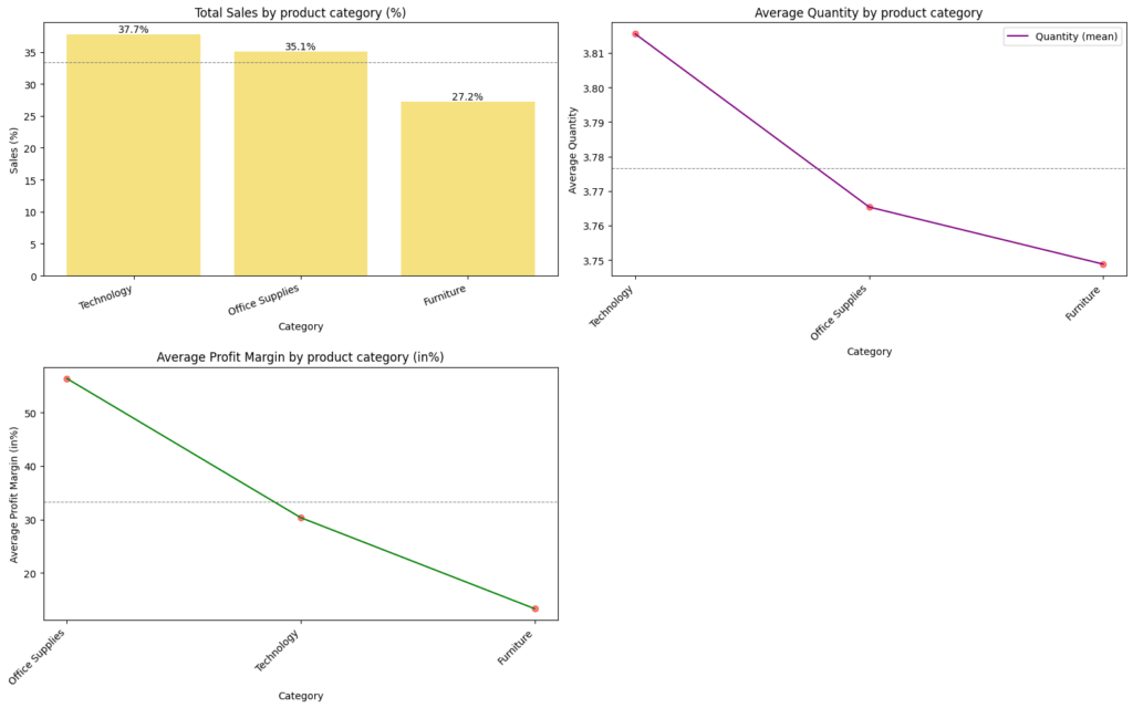
Target variables split by category

• Sales by Customer Product category (%): Technology have contributed over 37%, followed by office supplies and furniture
• Average Profit Margin by Product category(%): Average Profit margin equates to ~35%, of which office supplies stands at 55% margin
• Average Quantity by Product category: Average quantity is nearly 4 units

Target variables split by sub category

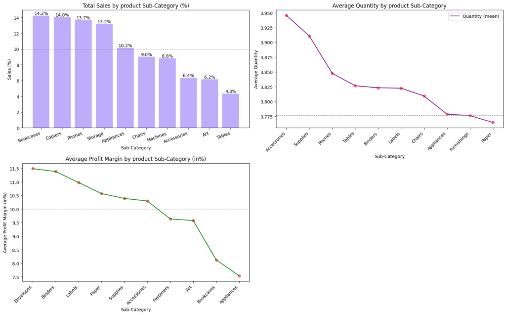
Target variables split by sub category

• Sales by Customer Product sub-category (%): Bookcases, Copiers, Phones, Storage and Appliance, contribute to ~65%
• Average Profit Margin by Product sub-category(%): Average Profit margin equates to 10%, ranging from 7.5 to 11.5% profit margin
• Average Quantity by Product sub-category: Average quantity is nearly 4 units

Target variables split by ship mode

Target variables split by ship mode

• Sales by Customer Product ship mode (%): Economy is the most preferred shipping mode followed by economy plus, priority and immediate
• Average Profit Margin by Product ship mode(%): Average Profit margin equates to 25%, ranging from 20 to 30% profit margin
• Average Quantity by Product ship mode: Average quantity is nearly 4 units

Address operational inefficiencies and customer engagement issues in underperforming areas

Sales percentage by Region vs Countries

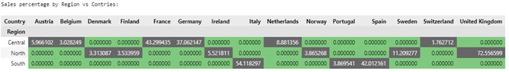
Sales percentage by Region vs Countries

• Region vs Countries: Underperforming countries (Sales less than 5%) are Belgium, Switzerland, Denmark, Finland, Norway and Portugal

Sales percentage by Countries vs State

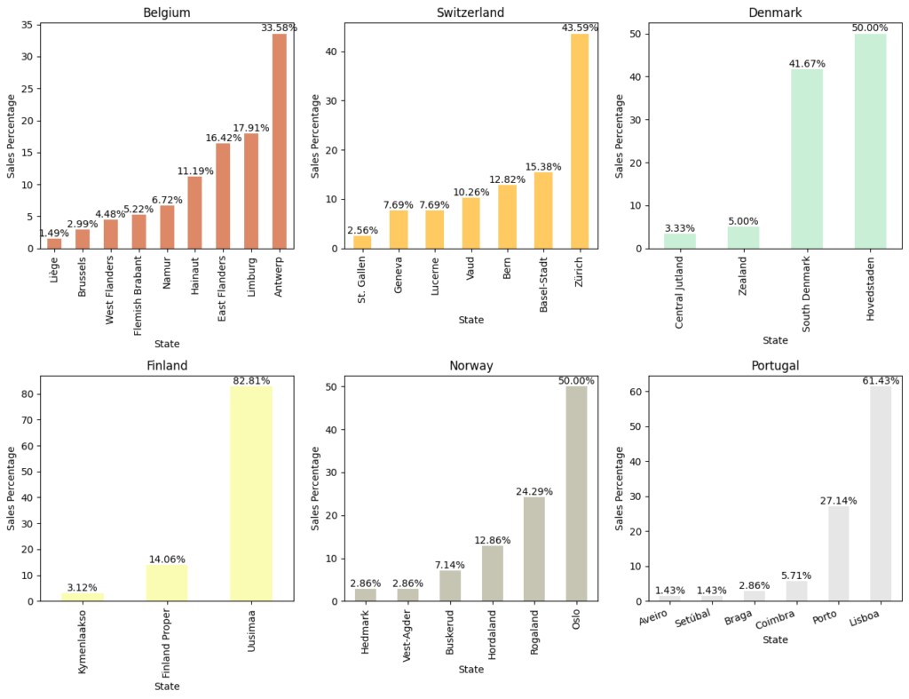
Sales percentage by Countries vs State

• Countries vs State: Underperforming counties are taken to deep dive to understand low performing states
• Under performing states (Sales less than 5%) in Belgium are, Liège, Brussels, West Flanders
• Under performing states (Sales less than 5%) in Switzerland is, St. Gallen
• Under performing states (Sales less than 5%) in Denmark are, Central Jutland, Zealand
• Under performing states (Sales less than 5%) in Finland is Kymenlaakso
• Under performing states (Sales less than 5%) in Norway are Hedmark, Vest-Agder
• Under performing states (Sales less than 5%) in Portugal are Aveiro, Setúbal, Braga

Sales percentage by State vs City

Sales percentage by State vs City

• State vs City: We notice that majority of underperforming states has only one branch in cityto cater to customer
• States with 2 cities are Liège, Braga
• States with 3 cities is West Flanders

Optimizing Discounts & Shipping Modes

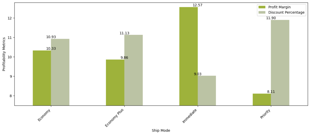
Profit margin vs Discount percentage:

• We could see that there is inverse relation among Discount percentage and Profit margin in Economy, Economy plus and priority mode
• In Immediate shipping mode, Discount is at lower side compared to profit margin, this could be because customers are willing pay more for quick product delivery

Sales, Profit, and Quantity by Discount Percentage

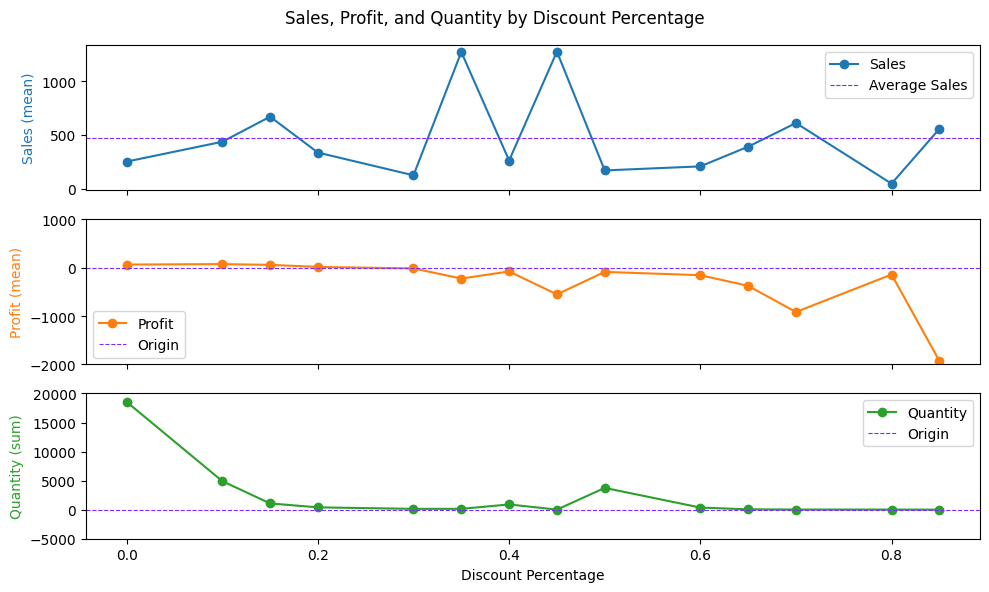
Sales, Profit, and Quantity by Discount Percentage

• Sales by Discount Percentage: Average sales stands at USD 500. Discount of 15%, 35%, 45%, 70% and 85% are having above average sales
• Profit margin by Discount Percentage: Average profit margin goes on decreasing as discount increases, when discount are more than 20% profit goes negative
• Quantity by Discount Percentage: When discount is from 0 to 20%, the sold quantity is higher compared to rest of discount offered

Feedback Analysis

Target variables split by feedback

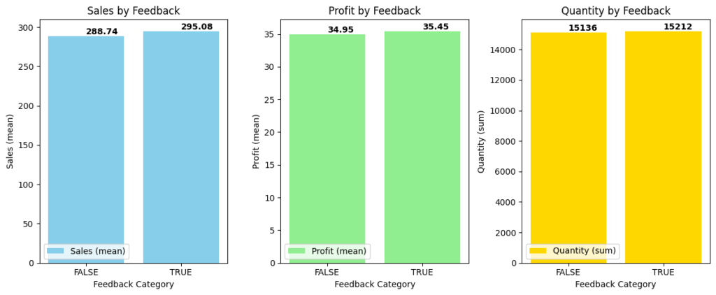
Target variables split by feedback

• We see that there is almost equal distribution of feedback provided among sales, profit and quantity

Top Products which received feedback

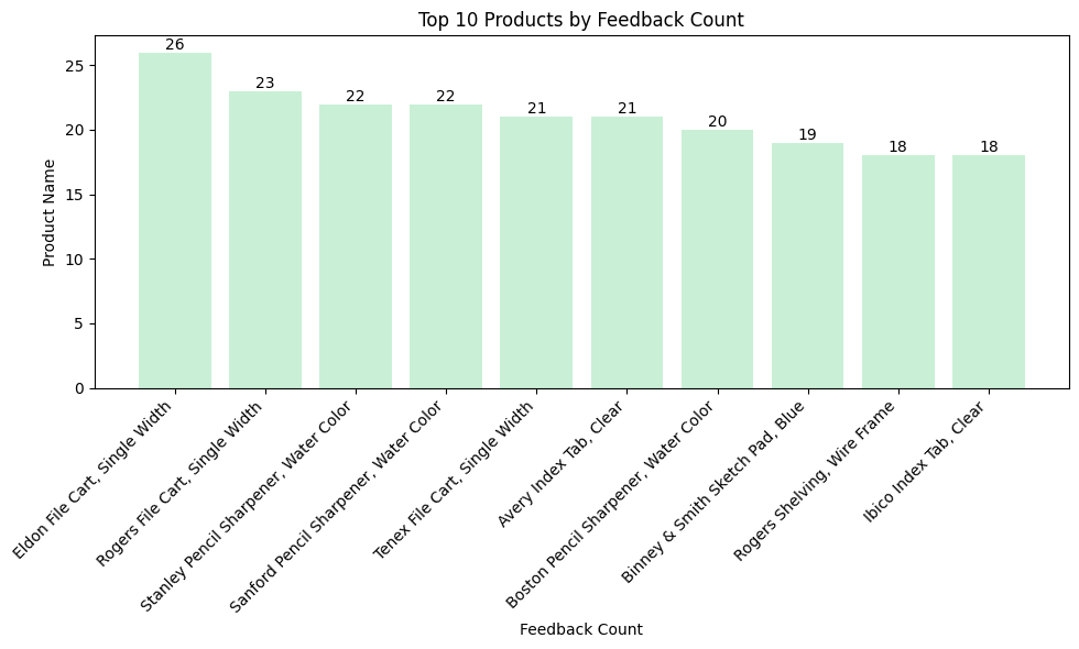
Top 10 Products by Feedback Count

• Eldon File Cart, Single Width is the most feedback received product, followed by Rogers File Cart, Stanley Pencil Sharpener, Sanford Pencil Sharpener… and so on

Top 10 Products with True & False Feedback

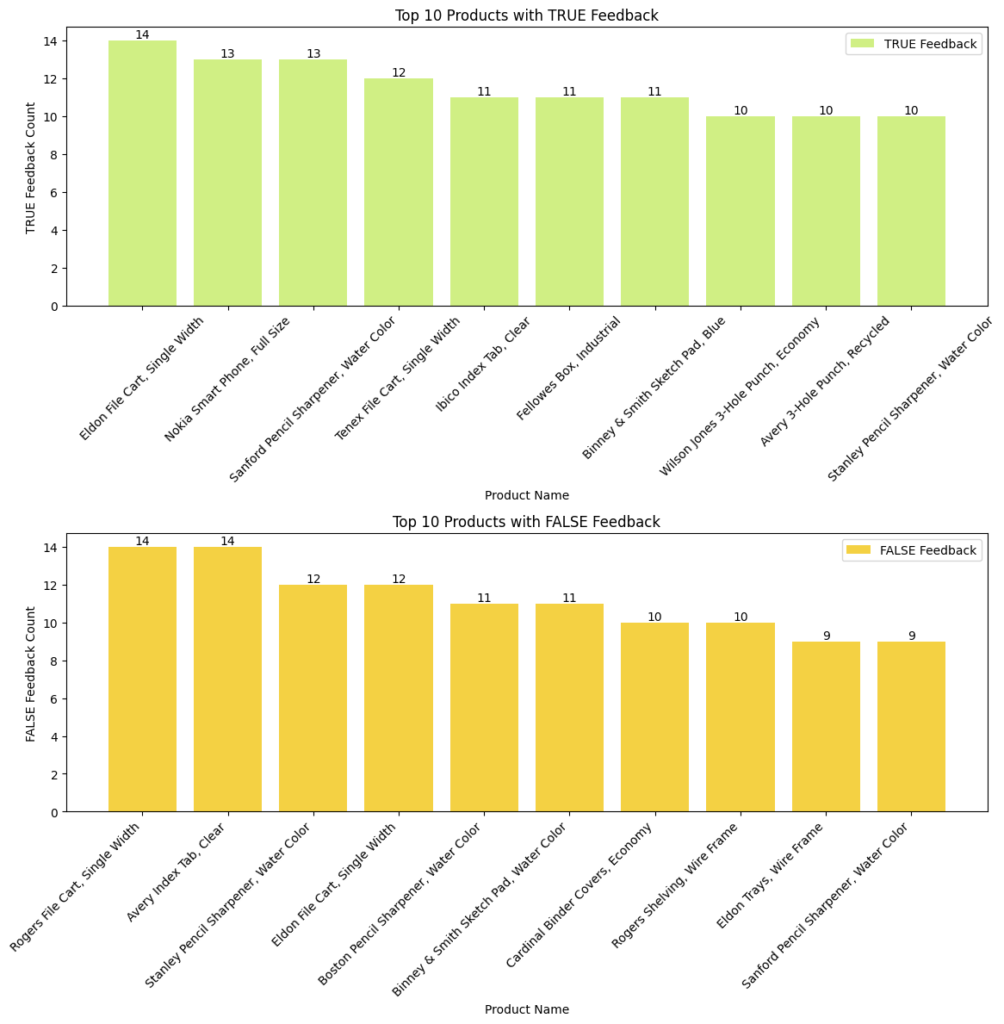
Top 10 Products with True & False Feedback

• Top Products with True Feedback
  • Eldon File Cart, Nokia Smartphone, Sanford Pencil Sharpener are the top 3 most products received True Feedback
• Top Products with False Feedback
  • Rogers File Cart, Avery Index Tab, Stanley Pencil Sharpener are the top 3 most products received False Feedback

Improving Product Mix

Top 10 Most product sales by value

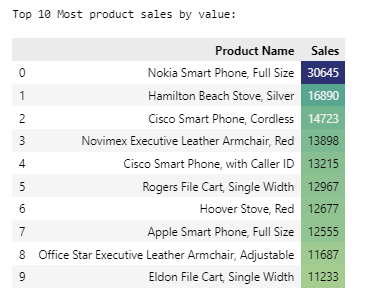
Top 10 Most product sales by value

• Nokia Smartphone, Hamilton Beach Stove, Cisco Smartphones are the top 3 most sales by value products

Top 10 Most Frequent Customers

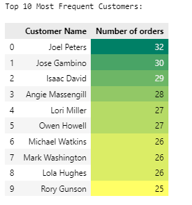
Top 10 Most Frequent Customers

• Joel Peters, Jose Gambino, Isaac David are the top 3 most loyal customers

Top 10 Most Profitable Products

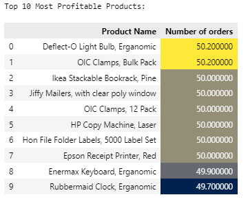
Top 10 Most Profitable Products

• Deflect-O Light Bulb, OIC Clamp, Ikea Stackable Book rack, Jiffy Mailers, HP Copy Machine, Hon File Folder Labels, Epson Receipt Printer are the top most profitable products with average profit margin by 50%

Top  most profitable category

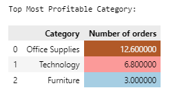
    Top  most profitable category

• Office supplies is the top most category which is most profitable, followed by technology and Furniture

Profitable Sub-Category

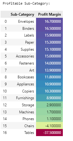
Profitable Sub-Category:

• Most of the sub-category products are having positive profit margin
• Chairs and Tables are having negative profit margin

Frequency of Order Sizes (Number of Products)

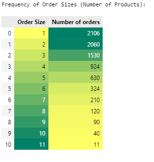
Frequency of Order Sizes (Number of Products)

• Order size 1 has the highest frequency with 2,160 orders
• Order size 11 has the lowest frequency with 40 orders
• As order size increases, the number of orders decreases

Commonly purchased product combinations (Order size 2)

Commonly purchased product combinations (Order size 2)

• Office Supplies with Office Supplies has highest sales combination
• Office Supplies with Technology has second-highest sales combination
• Furniture with Office Supplies has third-highest sales combination
• Furniture with Technology, Technology with technology and Furniture with furniture has low sales combination

Commonly purchased product combinations (Order size 3)

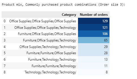
Commonly purchased product combinations (Order size 3)

• Office Supplies with Office Supplies with Office Supplies has highest sales combination
• Office Supplies with Office Supplies with Technology has second-highest sales combination
• Furniture, Furniture, Technology and Technology, Technology, Technology combination has low sales

Sales by quarter

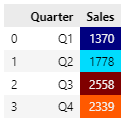
Sales by quarter

• Q3 and Q4 contributes to most sales in year

Sales by week

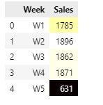
 Sales by week

• W1, W2, W3 and W4 contributes to most sales in a month

Chapter 5: Summary and Suggestions

Based on the analysis, here are my key summary and suggestions for Euromart to improve its business performance:

Identifying top performers

• Summary:
  • Regions: central region leads in sales (56%)
  • Countries: France, Germany, the UK, Italy, and Spain have strong sales contributions
  • States (top 10): England, france, and North Rhine-Westphalia contribute the most (66%). These states also boast positive profit margins (>9.25%)
  • Cities (top 10): London, Berlin, Vienna, Madrid, and Paris are top contributors with positive profit margins (9.8%-10.3%)
  • Customer segments: consumers account for most sales (52%), followed by corporate and home office. Their profit margins are also positive (30-35%)
  • Product categories: technology leads in sales (37%), followed by office supplies and furniture. Office supplies have the highest average profit margin (55%)
  • Economy is the most used shipping mode
  • Office supplies are dominant in the product category
• Suggestions:
  • Focus on top regions, increase marketing and promotional activities, logistics, and warehouses in France, Germany, and the UK to further boost sales
  • Segment-specific strategies, tailor marketing strategies for the consumer segment as it represents the largest customer base

Understanding challenges

• Summary:
  • Underperforming regions/countries: Belgium, Switzerland, Denmark, Finland, Norway, and Portugal have low sales (< 5%)
  • Underperforming states: several states within these countries have low sales
  • Low profitability: discounts above 20% lead to negative profits
  • Uneven city coverage: some underperforming states have only one branch
  • Negative feedback: some products receive negative feedback
  • Low order sizes: order size 1 has the highest frequency
  • Furniture and chairs: these categories have negative profit margins
• Suggestions:
  • Slowly expand the branches in under-performing countries to increase more reach to customers
  • Prioritize office supplies (highest profit margin) in underperforming areas to balance loss

Optimizing discounts & shipping modes

• Summary:
  • Higher discounts correlate with lower profit margins
  • Immediate shipping mode has lower discounts and higher profit margins, indicating customer willingness to pay for quick delivery
• Suggestions:
  • Optimize discount strategy, and reduce the extent of discounts above 20% to improve profit margins
  • Promote immediate shipping(Highest margins in shipping mode), highlight the benefits of immediate shipping to customers willing to pay more for faster delivery
  • Focus on promoting high-profit margin products

Leveraging customer feedback

• Summary:
  • Almost half of the customers have provided feedback
  • Specific products like eldon file cart and Nokia smartphone received significant feedback
• Suggestions:
  • Encourage more customers to provide feedback by offering incentives or simplifying the feedback process
  • Investigate products receiving no feedback and take actions to get feedback to improve the customer’s experience and identify potential issues faced

Improving product mix

• Summary:
  • Office supplies are the most profitable category
  • Chairs and tables have negative profit margins
  • Order size 1 is the most common, and as order size increases, the number of orders decreases
  • Certain product combinations are more popular than others based on order size
• Suggestions:
  • Refine product mix, focus on promoting and expanding the range of office supplies
  • Re-look at the pricing structure of chairs and tables as they have a negative profit margin
  • Encourage larger order sizes, upsell and cross-sell complementary products like office supplies with office supplies or office supplies with technology
  • Run promotions during high-selling times (Q3, Q4, first weeks of the month)

Additional recommendations

• Data-driven decision-making, continuously monitor sales, profit margins, and customer feedback to make data-driven decisions and adjust strategies accordingly
• Customer loyalty programs develop loyalty programs to reward top customers to encourage repeat purchases and enhance customer retention
• Efficiency improvements, streamline logistics and supply chain operations to reduce costs and improve delivery times, especially in underperforming regions

Annexure

Git hub link

https://github.com/VenuKumarM1/Euromart

Code snippets

Plotting Bar Graphs

• # We calculate frequency(count) of unique values in the column
• country_value_counts = df[‘Country’].value_counts()
• # We calculate percentage
• country_percentages = (country_value_counts / len(df)) * 100
• country_percentages
• # Creating the bar chart
• # Adjusting figure size for better readability
• plt.figure(figsize=(8, 6)) 
• # Setting color scheme for bars
• colors = [‘lightcoral’, ‘lightgrey’, ‘pink’, ‘gold’, ‘lightgreen’,
• ‘lightblue’,’lightcoral’, ‘skyblue’, ‘gold’, ‘skyblue’,
• ‘lightgreen’, ‘lightblue’, ‘skyblue’, ‘lightyellow’, ‘lavender’]
• # Creating bar chart with labels and title
• bars = plt.bar(country_value_counts.index, country_percentages, color=colors)
• plt.xlabel(“Country”)
• plt.ylabel(“Percentage (%)”)
• plt.title(“Distribution of Countries (with Percentages)”)
• # Adding percentages as text labels on top of bars
• for bar, perc in zip(bars, country_percentages):
• plt.text(bar.get_x() + bar.get_width() / 2, perc + 0.2, f”{perc:.1f}%”, ha=’center’, va=’bottom’);
• # Rotating x-axis labels for better readability
• plt.xticks(rotation=45, ha=’right’)
• # Adding gridlines on the x & y axis
• plt.grid(axis=’y’, linestyle=’–‘, alpha=0.7) 
• plt.grid(axis=’x’, linestyle=’–‘, alpha=0.7)
• # Adjusting space between chart
• plt.tight_layout()
• # Displaying the graph
• plt.show()

Plotting Pie chart

• # Getting the number of categories in variable
• segment_counts = df[‘Segment’].value_counts()
• # Pie chart
• # Adjusting figure size for better readability
• plt.figure(figsize=(3, 3))
• # Defining list to “explode” pie chart slices
• explode = [0.1, 0, 0]
• #Setting colours to the piechart slices
• colors = [‘lightgrey’, ‘lightblue’, ‘pink’]
• # Creating the pie chart
• plt.pie(segment_counts, labels=segment_counts.index, explode=explode, autopct=”%1.1f%%”, colors=colors)
• # Adding title to the chart
• plt.title(“Distribution of different customer segment”)
• # Displaying the chart
• plt.show()

Plotting box and whisker chart

• # Adding title to the chart
• ax1.set(title=’Distribution of discount in %’, ylabel=’count’)
• # Plotting the boxplot on the bottom subplot (ax2)
• ax2.boxplot(df[‘Discount Percentage’], labels=[‘All’], vert=False, showmeans=True, showfliers=True)  # Show means as diamonds & plot box plot
• # Adding title to the boxplot
• ax2.set(xlabel=’Discount Percentage’)
• #Display the summary statistics
• display(df[“Discount Percentage”].describe().round(2))

Plotting heat maps

• # Creating a figure and adjusting figure size for better readability
• fig, (ax1) = plt.subplots(1, figsize=(10, 5))
• # Calculating correlations of numerical datatypes
• correlation = df.select_dtypes(include=[np.number]).corr()
• # Creating a heatmap to visualize correlations
• sns.heatmap(correlation, annot=True, cmap=”PiYG”)  # Heatmap of correlations between numerical features
• # Adding title to the chart
• plt.title(“Correlation Heatmap”)
• # Displaying the graph
• plt.show()

Plotting Line chat

• # Subplot 3: Country vs Quantity (Line)
• # Positioning subplot at row 2, column 2, position 2
• plt.subplot(2, 2, 2)
• # Aggregate based on categories
• country_quantity = df.groupby(‘Country’)[‘Quantity’].mean()
• # Creating line chart with annotations
• plt.plot(country_quantity.index, country_quantity, color=’#E178C5′, label=’Quantity (mean)’)

• # Creating scatter plot to overalp on chart
• plt.scatter(country_quantity.index, country_quantity.values, color=’red’, alpha=0.5)
• # Plotting horizontal line represting average value
• plt.axhline(y=(country_quantity.values.mean()), color=’gray’, linestyle=’dashed’, linewidth=0.8)
• # Adding labels to the chart
• plt.xlabel(‘Country’)
• plt.ylabel(‘Average Quantity’)
• # Adding title to the chart
• plt.title(‘Average Quantity by Country’)
• # Rotating x-axis labels for better readability
• plt.xticks(rotation=45, ha=’right’)
• # Adding legend to the chart
• plt.legend()
• # Adjusting space between chart
• plt.tight_layout()
• # Displaying the graph
• plt.show()

Adding gradient to table

• # Region vs Countries
• # Printing a descriptive message to indicate the output
• print(“Sales percentage by Region vs Countries:”)
• # Creating a contingency table
• Regions_country = pd.crosstab([df[‘Region’]],
  • [df[‘Country’]],
  • values=df[‘Sales’],
  • aggfunc=’count’, normalize=”index”)*100
• # Displaying the table with background gradient styling for better readability
• display(Regions_country.style.background_gradient(cmap= “Accent”))